Using Neural Networks in Linguistic Resources
Cecilia Hemming
Department of Languages,
Introduction
This paper
is organised as follows:
Neural
Networks and Language Modeling.
Node
Functions in Hidden and Output Nodes
Neural
Nets and Speech Act Theory
Why Neural Nets?
An
interesting feature of neural nets is that knowledge can be represented at a
finer level than a single symbol (i.e., by means of several numbers), a
distributed description is therefore less prone to be corrupt. This method for
knowledge representation is known as sub-symbolic.
When there are difficulties to list or describe all symbols needed for an
adequate description by frames, semantic nets or logic, a neural net is very
useful: it works out the description for itself.
There are some
important differences when comparing connectionist techniques (known as neural
nets) with traditional, symbolic artificial intelligence. Symbolic AI
techniques are universal and especially good at searching for solutions by sequences
of reasoning steps. These traditional systems make use of structured design
methods, they have declarative knowledge which can be read and maintained by non-experts
but they are weak at simulating human common sense. Neural networks, on the
other hand, are good at perceptual optimising and common sense tasks but are
weak at logical reasoning and search. This sort of knowledge is not declarative
and can therefore not be inspected that easily. Symbolic and connectionist AI can
be seen as complementary approaches. (Bowerman, 2002)
What is a Neural Net?
The basic
idea underlying computational neural nets[1]
is that functions of the brain can be approximated with a computing system containing
a very large number of simple units. In analogy with biological nervous systems
these simple units are called neurons,
it is known that the human brain contains 1011of biological neurons.
A biological
cell consists of dendrites, a cell body, and an axon. The membrane covering the
cell body has a negative electric potential at its resting state. The synapses
(narrow gaps) transmit activations between the dendrites. Inputs through
excitatory synapses increases, and inputs through inhibitory synapses reduces, the
membrane potential. When the potential exceeds a threshold, a pulse is
generated. This pulse travels through the axon. The more inputs from excitatory
synapses a neuron receives, the more frequently it fires (i.e. sends an output
impulse).
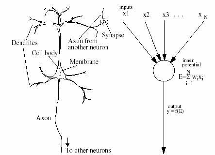
Figure 1. A biological neuron A
general artificial neuron
(Negishi, 1998)
A general computational
system has a labelled directed graph[2]
structure, see picture above. Each node performs some simple computations and
each connection conveys a signal from one node to another. All connections are
labelled with a number called the connection
strength or weight that indicates
to which extent a signal is amplified or diminished by the connection. Unlike
the biological original, the simplified artificial neuron is modelled under the
following assumptions:
- each node has only one output value,
distributed to other nodes via links
which
positions are irrelevant.
- all inputs are given simultaneously and
remain activated until the computation
of the
output function is completed.
- the position on the node of the incoming
connection is irrelevant.
(Mehrotra
et al., 1997:9)
The Perceptron
The
American researcher Frank Rosenblatt’s perceptron
for pattern classification is an early and one of the most known neural
networks, a very simplified description of it is here used to give an example
of the function of such a network.
This simple
perceptron has two layers of units, the input nodes (x1, x2)
and one output node, with weighted connections (w1, w2)
between them. The units take binary activity values (i.e. the pattern to
classify has to be encoded as a collection of binary values) and the final output
(y) will either be 0 or 1, which places the pattern in one of two classes (a
simple perceptron can only handle problems with just 2 answers, e.g. On/Off, Yes/No,
Left/Right).
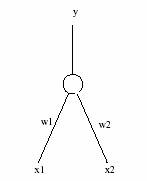
Output layer
Input layer
Figure 2. A
two-input perceptron with two adjustable weights and one output node
First, the
connections are assigned a weight at random, then, the weighted input for all
input nodes are summed up (in this case: x1w1 + x2w2) and
compared to a chosen threshold value. Possible input to this simple perceptron
is (0,0), (0,1), (1,0) or (1,1). The output function classifies each input
example according to its summed activity. In order to classify correctly, the
network can be trained. The training examples can therefore be assigned their
known desired output with which the actual output can be compared. Then by adjusting
the weights, the behaviour of the perceptron changes, so that the network eventually
generalizes over all examples and will be able to classify even new presented
patterns correctly, this is known as supervised
learning. Because the weights record cumulative changes, the order in which
the training patterns are presented does affect the search path through weight
space. To reduce the tendency for more recently presented patterns to
overshadow earlier patterns, the training set is repeated over many, so called,
epochs. An epoch refers to one
presentation of all examples in the training set.
Simple
perceptrons have a fundamental restriction, they can only induce linear
functions and thus not solve XOR-like problems[3].
(Werbos, 1974) was the first to propose a learning algorithm for networks with
more than two layers and with differentiable functions which solved such
problems (see the backpropagation
algorithm below). Several researchers in parallel rediscovered and
developed his work a decade later.
Neural Networks and Language
Modeling
The
simplest architecture for a neural network has a feedforward[4]
structure, in which information flows only in one direction: i.e. from the input
layer to the output layer, and in general via one or more layers of intermediate,
hidden[5], nodes. Such networks are very limited
in their ability to learn and process information over time, and that is why
they are not so well suited for language domains, that typically involve
complex temporal structure (Plaut, 1998). A better type of network for language
tasks has a recurrent structure, with no a priori constraints regarding in
which direction units can interact (Elman, 1991). Recurrent networks can also
learn to process sequences of inputs and/or to produce sequences of outputs.
For example, in a simple recurrent network like those proposed by Jeffrey Elman,
a representation of a given element of a sequence can be stored and reintroduced
as context information for subsequent elements, see schematic figure below.
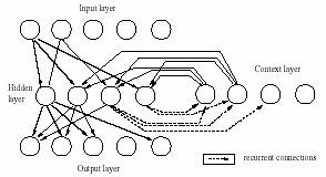
Figure 6. A
recurrent network with one hidden and one context layer, the latter is used as
a sort of memory.
(Kipp, 1998)
In many
linguistic theories context free and context sensitive components of language grammar
are separately represented by phrase structure at the one hand and some
labelling or slash notation at the other. But (Elman, 1991) stated that with
his neural network (that was used for word prediction) both could be
represented as context sensitive. As mentioned above, this was done through the
insertion of an intermediate context layer which is fed with a copy of each
hidden layer activity and then reintroduces this information back to the hidden
layer when the next input is presented. In this way the context and the current
input together are used to compute the next output and to update the context.
Modern
networks often use non-linear, proportional output and can thus cope with
problems which have more than two answers. Instead of the stepfunction used by the perceptron output node described above
(which according to a threshold value gives either “on” or “off” as an answer),
more complex functions that are differentiable can be used. The choice of node
functions that are differentiable everywhere allows the use of learning
algorithms based on gradient descent:
i.e. the weights are modified in small steps in a direction that corresponds to
the negative gradient of an error measure[6].
The backpropagation rule derived its
name from the fact that the errors made by the network are propagated back
through the network, i.e. the weights of the hidden layers are adapted
according to the error. The basic idea of the backpropagation (BP) algorithm is
that the error can be seen as a function of the weights (E = f(w) = f(w1,
w2, …, wn)). The different weights decide the output and
thereby also the errors, so the algorithm adjusts all weights in proportion to
their contribution to the output.
Node Functions
in Hidden and Output Nodes
Popular
node functions used in many neural nets are sigmoid
functions (see the graph of a sigmoid S-shaped curve below). They are continuous[7],
differentiable everywhere, rotationally symmetric about some point (net = 0, in the given example below) and they asymptotically approach their
saturation values (0 and 1 respectively, in the example below):
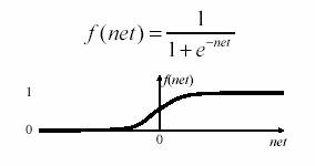
Figure 3. Graph
of a sigmoid function
For this
sigmoid function, when net (the net
weighted input to the node in question) is approaching ∞, the saturation
value for f(net) = 1, when net is approaching - ∞, the saturation value
for f(net) = 0 (the most common choices of f(net) saturation values for a
sigmoid function are 0 or -1 to 1). Other node functions, as the Gaussian or
Radial Basis functions, can be described as bell-shaped curves. Here f(net) has
a single maximum for net, which is the highest point of the bell-shaped curve. The
net value can also here be interpreted in terms of class membership, depending
on how close the net input is to the net maximum (i.e. the highest point of the
curve).
Mapping text to
speech sounds
In the late
eighties Rosenberg and Sejnowski developed a system for mapping English textual
words into corresponding speech sounds. This system, named NetTalk, uses a
neural network to convert a machine-readable text file to streams of symbols that
represent phonemes. A speech synthesiser was then used to turn the phoneme
representations into speech sounds.
One of the
networks used for this system was a feedforward multi-layer perceptron (MLP)[8]
with three layers of units and two layers of weighted connections in between
them. It was trained with the back-propagation algorithm. Input to the network was
a sequence of seven consecutive characters from an English text and the task
was to map the middle character (i.e. letter number four out of the totally seven)
to a representation of a single phoneme suitable in the context of the three characters
on each side of it. The network was trained until it generalized sufficiently and
then the connection weights were set to a fix value. The characters used were the
Roman alphabet letters plus three punctuation marks, see example below:
|
word |
phonemes |
Code for foreign and irregular words |
stress and syllable info |
|
abandon |
xb@ndxn0> |
1 |
<>0<0 |
|
abase |
xbes-0> |
1 |
<<0 |
|
abash |
xb@S-0> |
1 |
<<0 |
|
abattoir |
@bxt-+-r1<0<> |
2 |
<<2 |
Figure 4. Representation
of written words and phonemes in NetTalk (Sejnowski & Rosenberg, 1986).
For each of
the seven letter positions in the input, the network has a set of 29 input
units where the current character is represented as a pattern with only the
correspondent character unit activated ("on") and each of the others disactivated
("off").
On the
output side, there are 21 units that represent different articulatory features
such as voicing and vowel height. Each phoneme is represented by a distinct
binary vector over this 21 units set. Stress and syllable boundaries are encoded
in 5 additional output units.
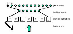
Figure 5. Input
character units and output phonemes of NetTalk (a second output for stresses
can be added).
(Jacobson, 2002)
A training set
with the 1000 most common English words, was tested with different net sizes,
i.e. with from zero up to 120 hidden units. The best performance with no hidden
units gave about 82% correct answers. An output was regarded as correct as long
as it was more close to the correct output vector than to any other phoneme
output vector. The more hidden units that were used, the better were the
learning rate and final performance of the net, 120 hidden nodes gave up to 98%
correct output. When the trained network was tested on a 20.000 word corpus
(without further training) it generated correct answers in 77% of the cases.
After five passes through this larger corpus 90% of the outputs were correct. (Sejnowski
& Rosenberg, 1986).
Neural Nets and
Speech Act Theory
Before the
work of Michael Kipp (Kipp, 1998) the problem of finding appropriate dialogue
acts for given utterances in large speech corpora was solved through symbolic,
decision tree and statistical approaches. Even if the latter showed the best
performance, problems due to the known sparse data effect of corpora limited
its usability. The corpus used in these experiments was a VERBMOBIL subcorpus
containing 467 German appointment scheduling dialogues.
An optimal
solution would be to assign each word to its proper input neuron but with the many
word tokens of the corpus this was proved far to time and power consuming. When
determining a dialogue act, information about the items part-of-speech (POS) is
valuable, e.g. when processing unknown words and also as it in some cases can
reveal a template-like structure: “How about <ADJECTIVE><NOUN>?” (suggest), “That <VERB> okay.” (accept) (Kipp, 1998). The final
design of the system comprised a multiple section vector with one segment for
each of the used POS-categories, yielding an input vector of 216 components as
described in the following. The POS-categories were divided into groups
according to their importance regarding the task. This enabled each POS-segment
to use its own representations for the words within it. In a POS of high importance
each word is represented by one distinct component. Within a medium-important
POS all words are represented by the binary value indicating their position in
the word list of the category. Words with low importance, finally, where the
interesting information is the category itself, cardinal numbers for instance,
were grouped to a single vector component lacking information about the
specific tokens (1, 20, 765, …etc. are all cardinal numbers but in this context
they give no specific individual information).
The network
system used, contained feedforward, partially recurrent network modules for
each POS and one selector network which gave the final dialogue act output. The
input was fed into the net by a sliding
window mechanism, this window sequentially scans the input
representations, thus allowing an utterance to be fed into the network moving
from the first part to the last, see figure on next page.
The choice
of solving this problem with the help of neural nets is due to the robustness
of these nets, the parallel and incremental processing and also because neural
nets automatically can be adapted to other, new, domains through training
(without extra hand-coding of new rules). In Kipp’s work there is no
comparison, though, with performances of systems using transformation-based
learning.
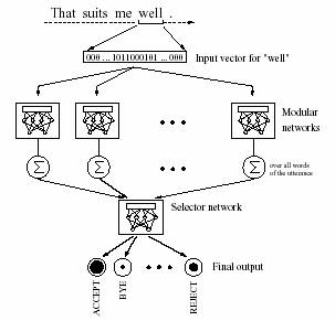
Figure 7. Kipp’s
network system showing the sliding input
window, the POS-selecting network modules and
the final
output selector network (Kipp, 1998).
Self-Organizing Maps
The
Self-Organizing Map (SOM), also called Kohonen Map from its inventor Teuvo
Kohonen, is one of the most widely used neural network algorithms. The learning
process is competitive and unsupervised, i.e. no desired output are involved in
the training of the net. The first layer
of a SOM is the input layer and each node in the second layer (often called the
Kohonen layer) is the winner for all
input vectors in a region of input space. Each jth node in the Kohonen
layer is described by the vector of weights to it from the input nodes: wj
= (wj1, wj2, …, wjn). Weight vectors have
the same dimension as input vectors and can thus be compared to these by a
distance measure estimating the similarity of them. A winner is the node whose
weight vector (w1, w2, …, wn) is nearest to an
input pattern. The weight vector associated with each node is as near as
possible to all input samples for which the node is the winner. At the same
time it is as far away as possible to very different samples.
A SOM can be visualized as a, most
often two-dimesional, coordinate system where the nodes are topologically ordered
according to a prespecified topology. The basic idea in its learning process is
that, for each sample input vector the winner and also, what is special for the
SOM, the nodes in the winners neighbourhood are positioned closer and closer to
the sample vector. Neighbours are nodes within a topological distance (the
length of the path connecting the nodes) from a node at a certain time, and the
training algorithm decreases this distance with time, as the training goes on. (Kohonen,
1997). Thus, in the beginning of the training phase all nodes tend to have
similar weights, close to average input patterns, but as the training proceeds
individual output nodes begins to represent different subset of input patterns.
(Honkela et
al. 1996) used the SOM to cluster averaged word contexts and then used this
data to organize documents in large document collections. Their corpus
contained 8800 articles from a Usenet newsgroup, with a total of 2 000 000
words. Non-textual information was first removed and numerical expression as
well as common code words were categorised into a few classes of special
symbols, seldom occurring words was removed and treated as empty slots. Common
general words were also removed from the corpus.
|
|
Figure 8. : The basic two-level WEBSOM architecture. a) The word category map first
learns to represent
relations of words based on
their averaged contexts. The word category map is used to form a word
histogram of the text to be analyzed. b) The
word category histogram is then used as input to the second SOM, the document
map. (Honkela et al. 1996)
The word
forms are first organized into categories on a word category map. With the help of this
map a word histogram of the text is formed. The document representation is
based on this histogram and explicitly expresses the similarity of
the word meanings. This information is then used to produce an organised document
map, which
provides a general two-dimensional view of the document collection.
This latter map has beeen adapted to A WWW-based environment, so that document
collections can be explored by a browser. The user may zoom at any map area by
pointing to the map image and thereby view the underlying document space in
more detail. The clustering between neighboring nodes is shown by using different
shades of gray, if the model vectors are close to each other, the shades are light,
if they are further apart they are darker. The WEBSOM browsing interface is
implemented as HTML- documents and can thus be viewed by a graphical WWW
browser. (Honkela et al.1996).
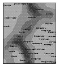
Figure 9. A part of a map for 20 newsgroups (Honkela
et al., 1996-2).
Conclusion
The
weaknesses and strengths of statistical and neural network approaches can be
further analysed, this to combine the two methods, e.g. in clustering dialogue
acts to groups and then specifying the members of them. Ideally, the clustering
should be based on automatically detected correlations, which neural nets are
good at finding.
By using
neural nets for mapping tasks, explicit combination of details and intricacies are
avoided. Rules for grammar, pronunciation and intonation are very complex and the
mapping from text to phonemes comprises combinatorial regularities with many
exceptions. Sejnowski and Rosenberg showed that the most important English pronunciation
rules could be captured in a context window of a few characters. Combinatorial
structures were captured through a distributed output representation (for
articulatory features and stress and syllable boundaries, respectively).
It seems
that the use of artificial neural network in language models offers a promising
methodology to explore linguistic resources of various kinds. Some applications
have been discussed in this paper but there is a lot of other interesting work in
this active field, as morpho-syntactic disambiguation, for instance (Vlasseva,
1999), (Simov & Osenova, 2001) or extended versions of the SOM, like token
category clustering, developed full-text analysis, information retrieval and
also interpretation of sign languages (Kohonen, 1997). An important application
of the SOM is to visualize very complex data and, as a clustering technique, to
create abstractions. The WEBSOM method has lately been further developed in
that the word category maps and also the number of documents classified have
been considerably enlarged, The largest map so far contains over one million
documents.
References
Bowerman,
C. 2002. School of Computing & Information Systems,
Elman, J.L. 1991. Distributed
representations, simple recurrent networks, and grammatical structure. Machine Learning, 7, 195–225.
Honkela, T., Kaski, S.,
Lagus K. and Kohonen T. 1996. WEBSOM - Self-Organizing Maps of
Document Collections.
Report.
Lagus K.,
Honkela, T., Kaski, K. and Kohonen T. 1996-2. WEBSOM - A Status Report. Proceedings of STeP'96. Jarmo Alander,
Timo Honkela and Matti Jakobsson (eds.),
Publications of the Finnish Artificial Intelligence Society, pp. 73-78.
Jacobsson, H. 2002. AI-neural nets,
lecture notes: lecture 4. Department of computer Science, University
College of Skövde.
Kipp, M. 1998.
The Neural Path to Dialogue Acts. In:
Proceedings of
the 13th European Conference on Artificial Intelligence (ECAI).
Kohonen, T. 1997. Self-Organizing Maps. 2nd edition. Springer Verlag, Heidelberg.
Malmgren, H. 2002. Nätverk för naturlig klassifikation.
http://www.phil.gu.se/ann (2002-03-03).
Manning,
C.D. and Schütze, H. 2001. Foundations of
Statistical Natural Language Processing. The MIT Press,
Mehrotra,
K., Mohan, C.K., Ranka, S. 1997. Elements
of Artificial Neural Networks. The MIT Press,
Negishi, M. 1998. Everything that Linguists have Always Wanted to Know about
Connectionism. Department of Cognitive and Neural Systems,
Sejnowski,
T. J. and Rosenberg, C. R. 1986. NETtalk: a parallel network that learns to
read aloud, Cognitive Science, 14,
179-211.
Simov,
K.I. & Osenaova, P.N. 2001. A Hybrid System for Morphosyntactic
Disambiguation in Bulgarian. BulTreeBank Project,
Vlasseva,
S. 1999. Part-Of-Speech Disambiguation in Bulgarian Language via Neural
Networks. Master’s Thesis. Faculty of Mathematics and Computer Science, st.
Kl. Ohridsky University,
Werbos, P.
1974. Beyond regression: new tools for
prediction and analysis in the behavioural sciences. PhD thesis,